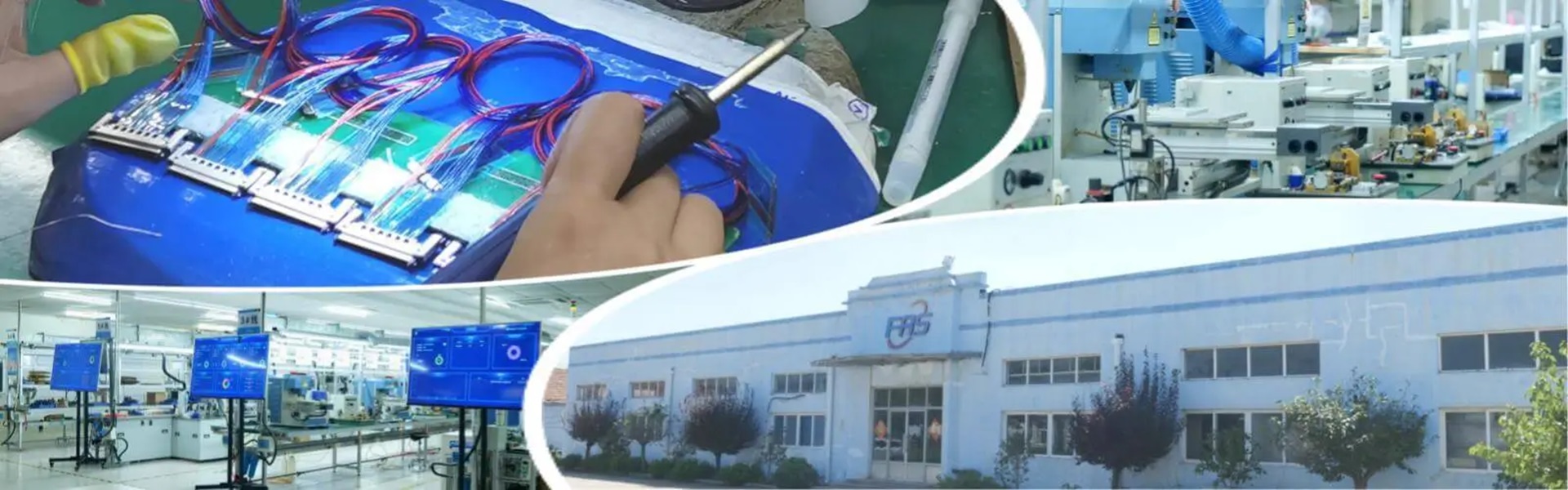
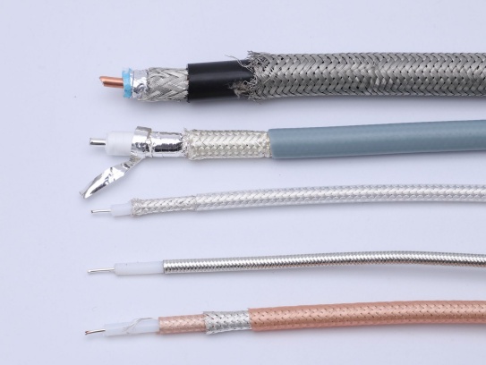
RF Micro Coaxial Cable
Meta Description: Discover premium RF micro coaxial cables engineered for high-frequency signal transmission in compact devices. Explore specs, applications, and benefits for telecom, medical, and aerospace industries. .
1. Impedance in Micro Coaxial Cables
Impedance, measured in ohms (Ω), defines the cable’s resistance to alternating current (AC) signals. Proper impedance matching minimizes signal reflections and ensures maximum power transfer.
Standard Impedance Values
50 Ω:
Design Focus: Optimized for RF and microwave systems (e.g., radar, cellular networks).
Advantages: Balances power handling and low loss at high frequencies.
Typical Use Cases: 5G antennas, satellite transceivers, and vector network analyzers (VNAs).
75 Ω:
Design Focus: Tailored for video and broadband signals (e.g., HDTV, CCTV).
Advantages: Lower capacitance per unit length, ideal for long-distance analog transmission.
Typical Use Cases: Endoscopes, broadcast cameras, and automotive infotainment.
Custom Impedances (e.g., 93 Ω, 100 Ω):
Design Focus: Niche applications like high-speed digital interconnects (PCIe, USB4).
Advantages: Matches PCB trace impedances to reduce crosstalk.
Factors Affecting Impedance
Conductor Diameter: Larger inner conductors lower impedance.
Dielectric Constant (Dk): Lower Dk materials (e.g., ePTFE) increase impedance.
Shield Geometry: Tight braiding or foil layers slightly reduce impedance.
2. Frequency Range: Pushing the GHz Barrier
Micro coaxial cables are designed to operate across broad frequency spectrums, from DC to millimeter-wave (mmWave) bands.
Key Determinants of Frequency Range
Dielectric Material:
Low-loss dielectrics like expanded PTFE (Dk ≈ 1.3) support frequencies up to 110 GHz.
Example: A 0.81 mm cable with ePTFE achieves 0.1 dB/cm loss at 60 GHz.
Skin Effect Mitigation:
Silver or gold plating on conductors reduces resistance at high frequencies.
Shielding Effectiveness:
Multi-layer shields (foil + braid) minimize leakage and sustain performance above 40 GHz.
Frequency-Dependent Loss
Attenuation (dB/m): Increases with frequency due to dielectric and conductor losses.
Formula:
=
conductor
+
dielectric
∝
α=α
conductor
+α
dielectric
∝
f
.
Phase Stability: Critical for phased-array systems; high-purity dielectrics ensure linear phase response.
3. Impedance vs. Frequency Trade-offs
Designing micro coax involves balancing impedance stability with frequency capabilities:
Parameter 50 Ω Cable 75 Ω Cable
Optimal Frequency 1–100 GHz DC–6 GHz
Power Handling High (≈100 W) Moderate (≈10 W)
Loss @ 10 GHz 0.2 dB/cm 0.5 dB/cm
Common Applications RF frontends, VNAs Video transmission, IoT sensors
Note: 50 Ω cables dominate high-frequency applications, while 75 Ω excels in cost-sensitive, lower-frequency systems.
4. Testing and Calibration
Ensuring impedance and frequency specifications requires rigorous testing:
Time-Domain Reflectometry (TDR):
Measures impedance variations along the cable length.
Vector Network Analyzer (VNA):
Characterizes S-parameters (e.g., S11 for reflections, S21 for insertion loss).
Phase-Gain Analyzers:
Validate phase linearity for radar and beamforming systems.
5. Application-Specific Design Examples
6G Prototyping (300 GHz):
Cable: 0.3 mm diameter, 50 Ω, air-core dielectric.
Performance: Supports 0.15 dB/cm loss at 300 GHz.
Medical Ultrasound (15 MHz–20 MHz):
Cable: 1.2 mm diameter, 75 Ω, FEP dielectric.
Performance: Maintains 75 Ω ±2% across 100+ flex cycles.
Automotive Radar (77 GHz):
Cable: 0.9 mm diameter, 50 Ω, ePTFE dielectric.
Performance: VSWR <1.2:1 up to 110 GHz.
6. Future Trends
Impedance-Tunable Cables:
Materials with voltage-dependent Dk (e.g., liquid crystals) for adaptive impedance matching.
THz-Frequency Cables:
Sub-0.2 mm cables using graphene conductors and metasurface shields.
AI-Optimized Designs:
Machine learning algorithms to predict impedance/frequency performance for custom geometries.
Meta Description: Discover premium RF micro coaxial cables engineered for high-frequency signal transmission in compact devices. Explore specs, applications, and benefits for telecom, medical, and aerospace industries. .
Micro Coaxial Cable: High-Quality Solutions for Precision Applications Micro coaxial cables are essential components in high-performance electronic applications, providing reliable signal transmission in compact and flexible designs. A.
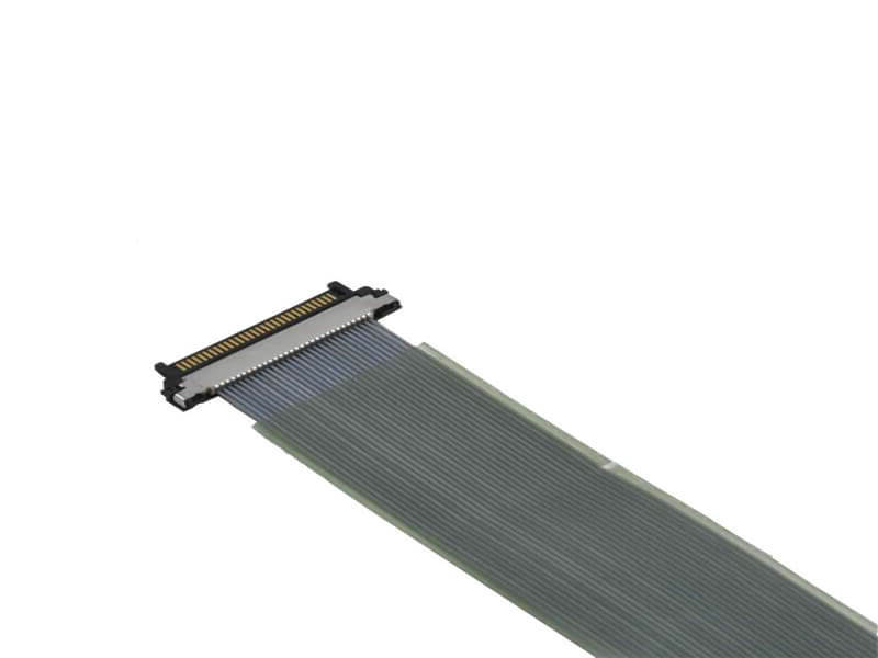
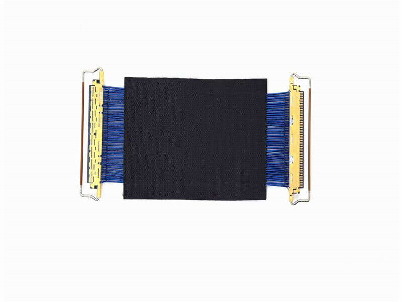
KEL’s Micro Coaxial Cable solutions are at the forefront of modern electronic connectivity, offering exceptional performance in high-speed data transmission, miniaturization, and reliability. These connectors are integral to various.
Overview of I-PEX Micro Coaxial Cable Connectors I-PEX is a global leader in micro coaxial cable solutions, specializing in high-performance IPEX micro coax connectors and micro coaxial cable assemblies. These products are designed for.
In LVDS (Low Voltage Differential Signaling) display systems, Micro-coaxial Cable (also referred to as Micro Coax Cable) stands out as an optimal solution for high-resolution, high-reliability signal transmission. Designed to meet the str.